15  Foundation forecasting models

Load common libraries and settings
import warnings
warnings.filterwarnings("ignore")
import os
os.environ["NIXTLA_ID_AS_COL"] = "true"
import numpy as np
np.set_printoptions(suppress=True)
np.random.seed(1)
import random
random.seed(1)
import pandas as pd
pd.set_option("max_colwidth", 100)
pd.set_option("display.precision", 3)
from utilsforecast.plotting import plot_series as plot_series_utils
import seaborn as sns
sns.set_style("whitegrid")
import matplotlib.pyplot as plt
plt.style.use("ggplot")
plt.rcParams.update({
    "figure.figsize": (8, 5),
    "figure.dpi": 100,
    "figure.constrained_layout.use": True,
    "font.size": 11.5,
    "axes.titlesize": 14,
    "axes.labelsize": 11.5,
    "xtick.labelsize": 10.5,
    "ytick.labelsize": 10.5,
    "legend.fontsize": 9.5,
    "legend.title_fontsize": 11.5,
    "grid.alpha": 1.0,
})
import matplotlib as mpl
from cycler import cycler
mpl.rcParams['axes.prop_cycle'] = cycler(color=["#000000", "#000000"])
from fpppy.utils import plot_series

mpl.colormaps.register(
    mpl.colors.ListedColormap(
        ["#000000", "#2f2fff"], name="black_and_blue"),
    force=True,
)
mpl.colormaps.register(
    mpl.colors.ListedColormap(
        ["#000000", "#D55E00"], name="black_and_orange"),
    force=True,
)
mpl.colormaps.register(
    mpl.colors.ListedColormap(
        ["#000000", "#000000"], name="black"),
    force=True,
)
mpl.colormaps.register(
    mpl.colors.ListedColormap(
        ["#000000", "#0072B2", "#D55E00"],
        name='black_and_2color',
    ),
    force=True
)
mpl.colormaps.register(
    mpl.colors.ListedColormap(
        ["#000000", "#D55E00", "#0072B2", "#009E73"],
        name='black_and_3color',
    ),
    force=True
)
mpl.colormaps.register(
    mpl.colors.ListedColormap(
        ["#000000", "#D55E00", "#0072B2", "#009E73", "#CC79A7"],
        name='black_and_4color',
    ),
    force=True
)
mpl.colormaps.register(
    mpl.colors.ListedColormap(
        ["#D55E00", "#0072B2", "#009E73", "#CC79A7"],
        name='r_colors',
    ),
    force=True
)
Load additional libraries
from IPython.display import Image
from datasetsforecast.m4 import M4
from neuralforecast.core import NeuralForecast
from neuralforecast.models import NHITS
from neuralforecast.utils import AirPassengersDF
from nixtla import NixtlaClient
from utilsforecast.evaluation import evaluate
from utilsforecast.losses import mae

from gluonts.dataset.pandas import PandasDataset
from gluonts.dataset.split import split
from uni2ts.model.moirai import MoiraiForecast, MoiraiModule

15.1 Introduction

In recent years, advancements in Neural Networks (NNs), particularly transformer-based models, have gained attention in time series forecasting. Building on work from other domains, research has grown rapidly in applying NNs to time series tasks. As explained in Chapter 14, the main appeal comes from their ability to automatically extract meaningful representations from raw data, enabling them to capture complex nonlinear relationships in temporal dependencies.

Transformers and Attention Mechanisms

One of the most influential developments in deep learning has been the transformer architecture, introduced in Attention Is All You Need (Vaswani et al., 2017). Unlike traditional recurrent neural networks (RNNs) or long short-term memory (LSTM) networks, transformers process entire input sequences in parallel rather than sequentially. This eliminates the need for step-by-step recurrence, making them more scalable and efficient for large datasets.

The key innovation in transformers is the self-attention mechanism, which allows the model to weigh the importance of different input elements, even when they are far apart in a sequence. This makes transformers particularly effective for capturing long-range dependencies, a crucial advantage in domains like natural language processing (NLP) and time series forecasting. By leveraging multiple layers of self-attention and feed-forward networks, transformers learn complex hierarchical representations of data, making them powerful tools for various sequential tasks.

Foundation Models and Their Impact

Foundation models, including large language models (LLMs) in natural language processing, have transformed AI by achieving state-of-the-art performance across diverse applications. These models leverage extensive datasets to build generalised representations, allowing them to perform well in a zero-shot fashion—making predictions without being specifically trained on a particular dataset. This paradigm eliminates the need to develop, implement, and train task-specific models for each use case.

The concept of foundation models gained prominence with BERT (Devlin et al., 2019) and GPT (Radford & Narasimhan, 2018), but it was GPT-3 (Brown et al., 2020) that demonstrated their full potential. Unlike earlier models that required task-specific supervised learning, foundation models follow a semi-supervised pre-training framework, where they first learn general patterns from vast amounts of unlabelled data and then adapt to specific tasks through fine-tuning.

While this approach revolutionised NLP, it has since been extended to other domains. In computer vision, models like Vision Transformers (Dosovitskiy et al., 2021) have applied transformer-based architectures to image processing. In scientific applications, foundation models such as AlphaFold (Jumper et al., 2021) have significantly advanced protein structure prediction.

Given the success of foundation models in natural language processing and computer vision, researchers have explored their application in time series forecasting. A notable early work by (Oreshkin et al., 2021) demonstrated that the N-BEATS model could be pre-trained to enable zero-shot forecasting.

Potential advantages

Foundation models offer key benefits over traditional task-specific approaches in time series forecasting. While this technology remains in early stages, its advantages include:

  • Ease of use: Foundation models are pre-trained on large-scale datasets, allowing direct application to new datasets without extensive training.
  • Lower computational requirements: They reduce computational costs by eliminating intensive training on individual datasets.
  • Accuracy with limited data: Foundation models excel with limited data. Their extensive pre-training helps capture underlying patterns that data-specific models often miss with limited training data.

Overall, foundation models represent a significant shift in time series forecasting, providing a flexible and scalable alternative to traditional methods. As research continues to evolve, these models have the potential to redefine forecasting across various industries.

15.2 Transfer learning

Foundation models rely on their capabilities to generalise across domains, particularly in new tasks that were not available during training. We understand, accordingly, transfer learning as the capacity to apply knowledge gleaned from one task to solve new tasks.

A forecasting model provides a function f_\theta : X \mapsto Y, with X the feature space and Y the dependent variable space. We consider the setting with X = \{y_{[0:t]}, x_{[0:t+h]}\} and Y = \{y_{[t+1:t+h]}\}, where h is the forecast horizon, y is the target time series, and x are exogenous covariates. The forecasting task objective is to estimate the following conditional distribution: P(y_{[t+1:t+h]} | y_{[0:t]}, x_{[0:t+h]}) = f_\theta (y_{[0:t]}, x_{[0:t+h]}) \tag{1} Transfer-learning refers to pre-training a model on a (usually large) source dataset to improve its performance on a new forecasting task with a target dataset.

The core idea of a foundation model is to leverage this principle by training a model on a large time series dataset, leveraging scaling laws on the dataset and model sizes. A diverse dataset, in terms of breadth and depth, is necessary for the model to perform in a wide variety of domains.

Example: Transfer-learning from M4 to Air Passengers

In the following simple example we illustrate this process by pre-training the NHITS (Challu et al., 2023) on the M4 monthly dataset. The M4 dataset is a collection of 100,000 time series used for the fourth edition of the Makridakis forecasting Competition (Makridakis et al., 2020). The M4 dataset consists of time series of yearly, quarterly, monthly and other (weekly, daily and hourly) data, which are divided into training and test sets. The M4 dataset was created by selecting a random sample of 100,000 time series from the ForeDeCk database. The selected series were then scaled to prevent negative observations and values lower than 10, thus avoiding possible problems when calculating various error measures. The scaling was performed by simply adding a constant to the series so that their minimum value was equal to 10 (29 occurrences across the whole dataset). In addition, any information that could possibly lead to the identification of the original series was removed to ensure the objectivity of the results.

Y_df = M4.load(directory="data", group="Monthly")[0].assign(
    ds=lambda df: df.groupby("unique_id")["ds"].transform(lambda x:
        pd.date_range(start="1970-01-01", periods=len(x), freq="MS")
    )
)
Y_df.head()
unique_id ds y
0 M1 1970-01-01 8000
1 M1 1970-02-01 8350
2 M1 1970-03-01 8570
3 M1 1970-04-01 7700
4 M1 1970-05-01 7080
horizon = 12
stacks = 3
models = [
    NHITS(
        input_size=5 * horizon,
        h=horizon,
        max_steps=2_000,
        stack_types=stacks * ["identity"],
        n_blocks=stacks * [1],
        mlp_units=[[256, 256] for _ in range(stacks)],
        n_pool_kernel_size=stacks * [1],
        batch_size=32,
        scaler_type="standard",
        n_freq_downsample=[12, 4, 1],
    )
]
nf = NeuralForecast(models=models, freq="MS")
nf.fit(df=Y_df)

Then, we can use the pre-trained model to forecast the air_passengers dataset, unseen during training.

air_passengers_df = AirPassengersDF.copy()
transfer_preds = nf.predict(df=air_passengers_df)
plot_series(air_passengers_df, transfer_preds,
    xlabel="Month", ylabel="Number of passengers",
    title = "International airline passengers",
    palette="black_and_blue", rm_legend=False,
    legend_loc="outside lower center")

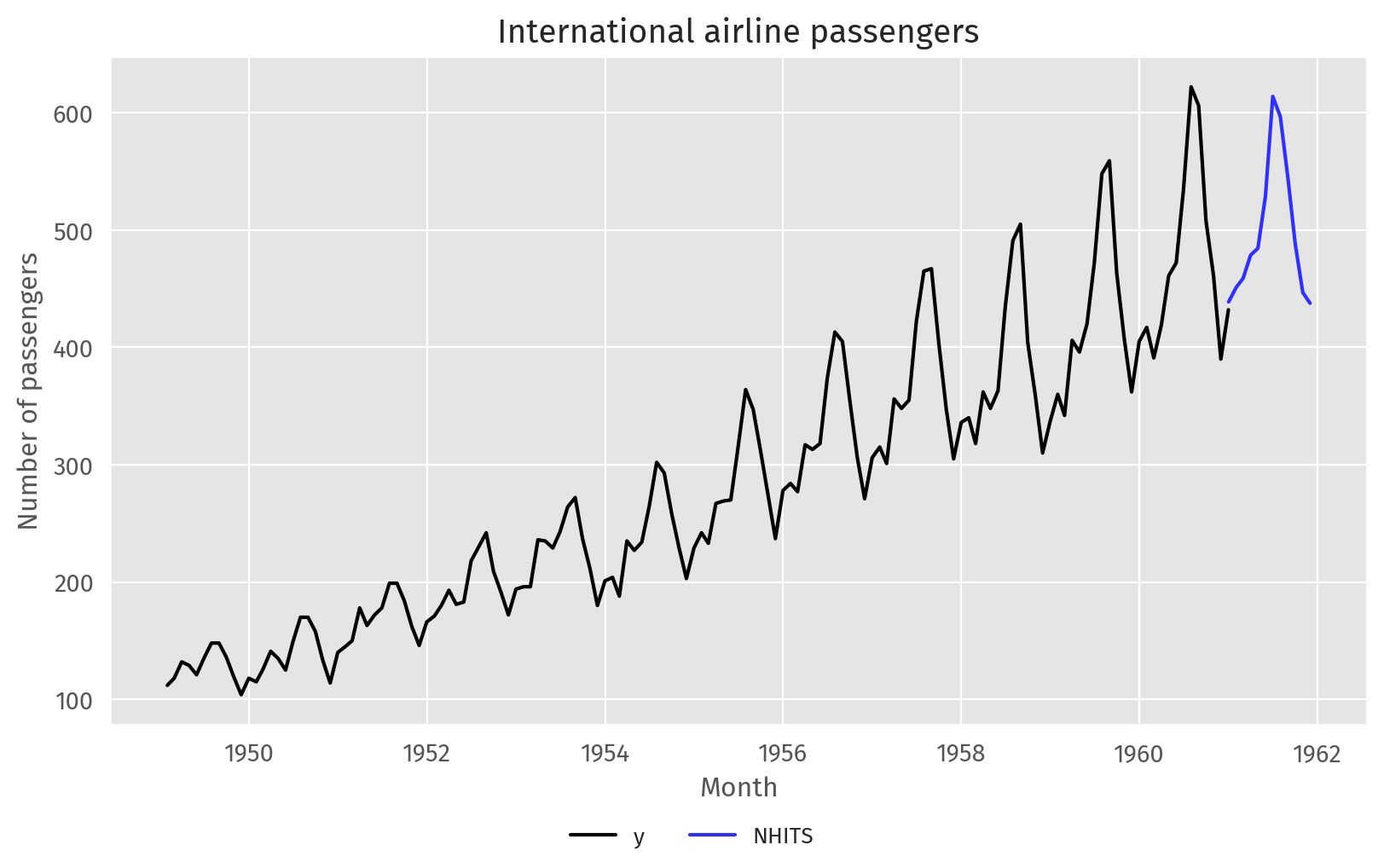
Figure 15.1: Forecasts by transfer learning.

In Figure 15.1, we can see that the model, despite not being trained on this particular dataset, is able to generate forecasts that capture the overall behaviour of the series.

15.3 Overview of foundation models

Foundation models represent a paradigm shift in the field of forecasting, enabling the application of pre-trained models to a wide range of time series tasks without the need for dataset-specific training. This approach, still in its early stages, has generated significant attention, leading to the development of multiple models. Below is a chronological overview of notable foundation models:

Next, we present an overview of some of these models. Understanding the core components of the transformer is required to understand the particularities of each large time model. We suggest you read The Illustrated Transformer if you are not comfortable with some of the following terms and concepts.

TimeGPT

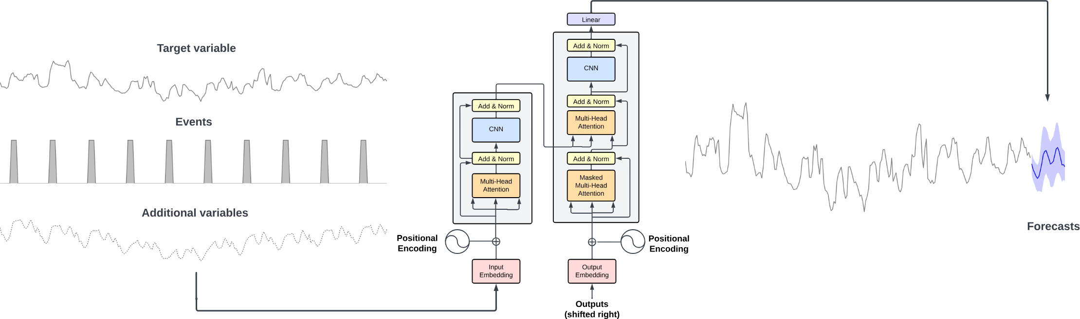
Figure 15.2: Architecture of TimeGPT.

TimeGPT is a transformer-based time series model that uses self-attention mechanisms, a method that allows the model to weigh the importance of different past observations when making a forecast. Instead of treating all past values equally, self-attention assigns different levels of importance based on how relevant each point is to the current prediction. TimeGPT takes a window of historical values as input and enhances it with local positional encoding, a technique that provides information about the order of data points—critical for understanding time-dependent patterns. The architecture follows an encoder-decoder structure, where the encoder processes input time series and extracts relevant features, while the decoder uses this processed information to generate forecasts. Each layer in the model includes residual connections (which help preserve information and improve training stability) and layer normalisation (which standardises activations to ensure stable learning). Finally, a linear layer maps the decoder’s output to match the desired forecast horizon. The general intuition behind attention-based models is their ability to learn from diverse past events and extrapolate potential future distributions based on patterns observed in historical data.

TimeGPT was trained on a large collection of publicly available time series, collectively encompassing over 100 billion data points. This training set incorporates time series from a broad array of domains, including finance, economics, demographics, healthcare, weather, IoT sensor data, energy, web traffic, sales, transport, and banking.

For more information:

Lag-Llama

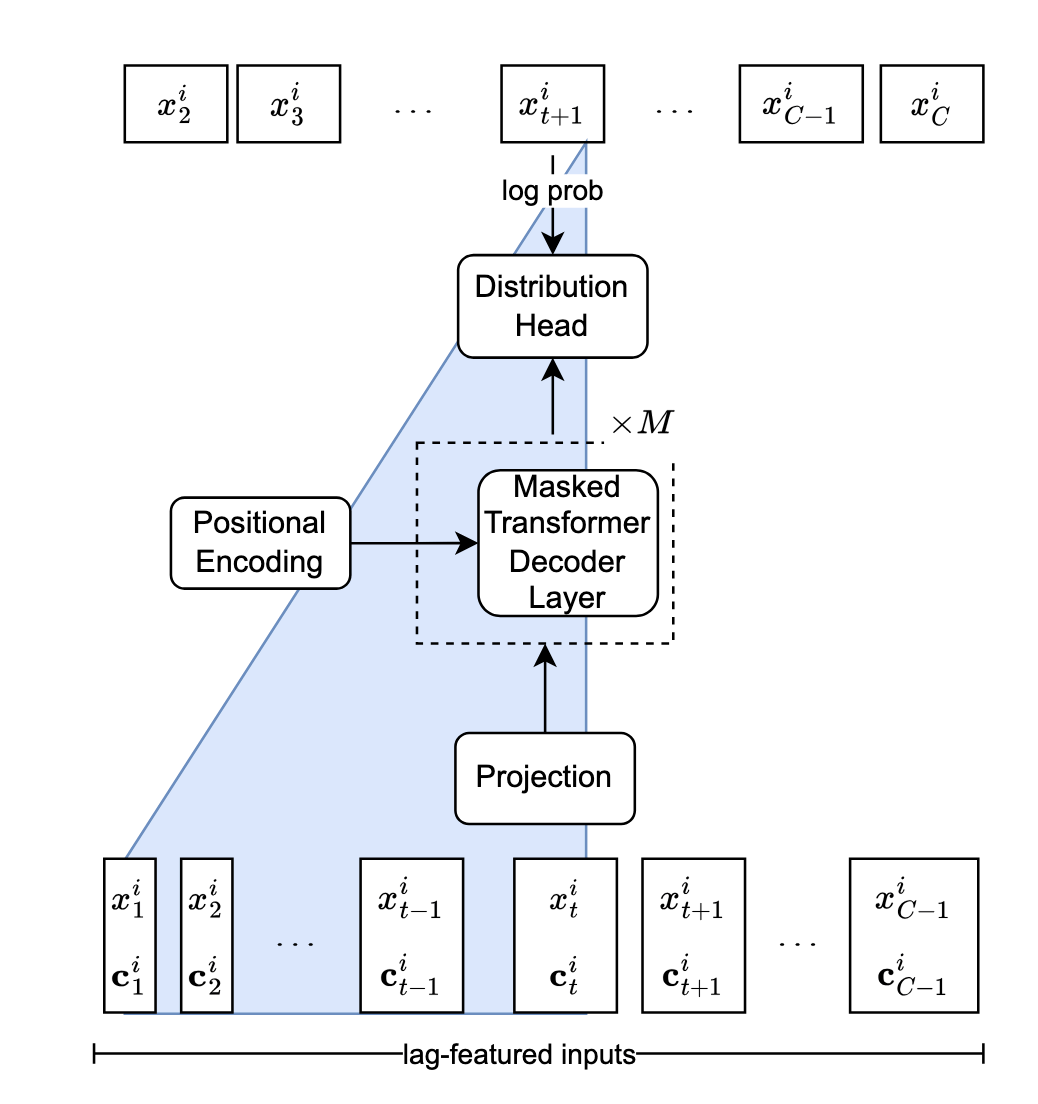
Figure 15.3: Architecture of Lag-Llama.

Lag-Llama is a probabilistic univariate forecasting model. It is a decoder-only transformer, meaning it does not use an encoder to preprocess the data; instead, it directly generates the forecast. The model builds lagged features, which are previous time series values that serve as inputs to the model. For example, it extracts seasonal indicators such as the quarter, month, day of the week, and finer-grained time elements down to the second. This helps the model capture seasonal patterns and short-term fluctuations. To estimate uncertainty in its predictions, Lag-Llama assumes a Student’s t-distribution.

For more information:

TimesFM

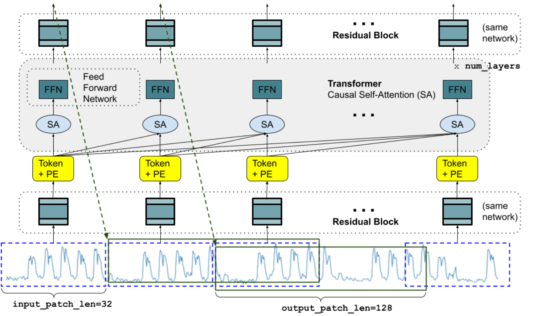
Figure 15.4: Architecture of TimesFM.

TimesFM is decoder-based foundation model developed by Google Research. It is a deterministic model focusing on point forecasts. It relies on patching the series to extract local semantic information from groups of data points. The model patches the input series and is trained to output longer output patches, such that it undergoes fewer autoregressive steps if the forecast horizon exceeds the output patch length. It uses a decoder-only transformer and uses a residual block to embed the input series and map the output of the decoder to predictions.

For more information:

Tiny Time Mixers

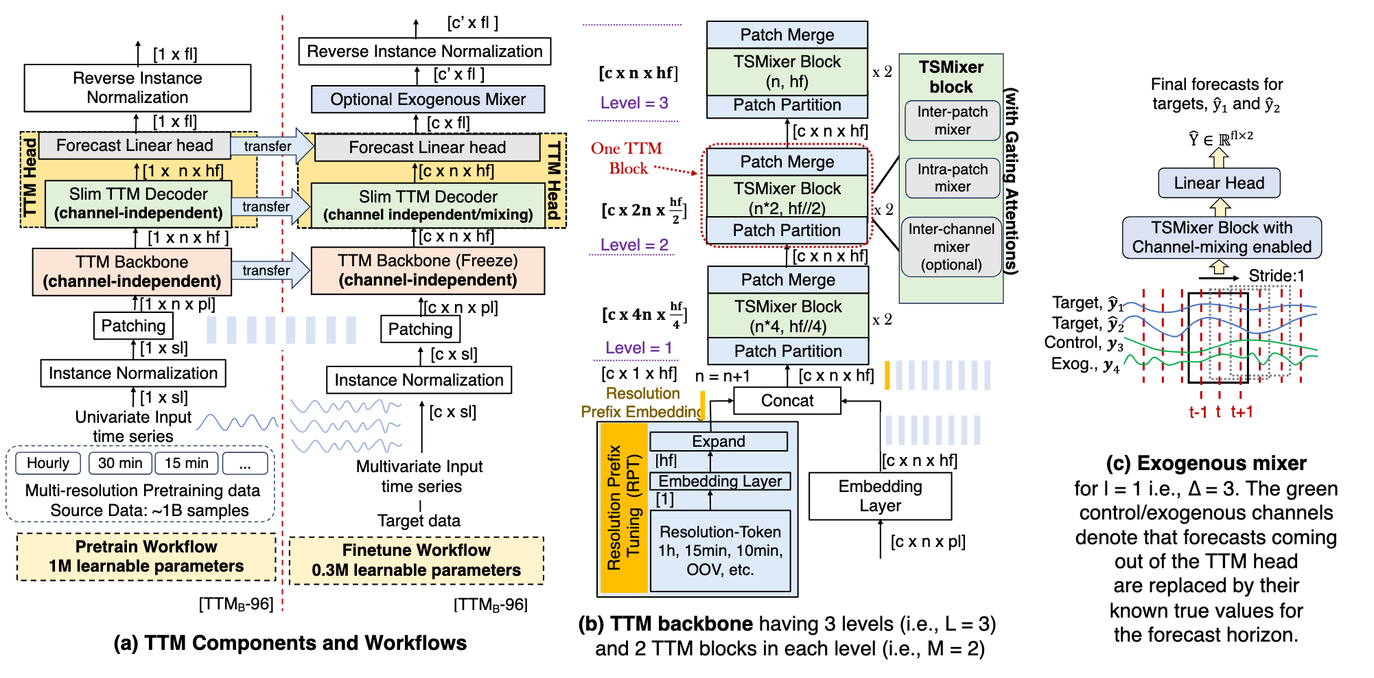
Figure 15.5: Architecture of Tiny Time Mixers.

Tiny Time Mixers (TTM) is a lightweight model (starting at 1M parameters) based on the TSMixer architecture, and developed by IBM Research. The objective was to build a small foundation model that could run on CPU-only machines and reduce computational requirements. It is also a deterministic model and it supports exogenous features.

For more information:

Moirai

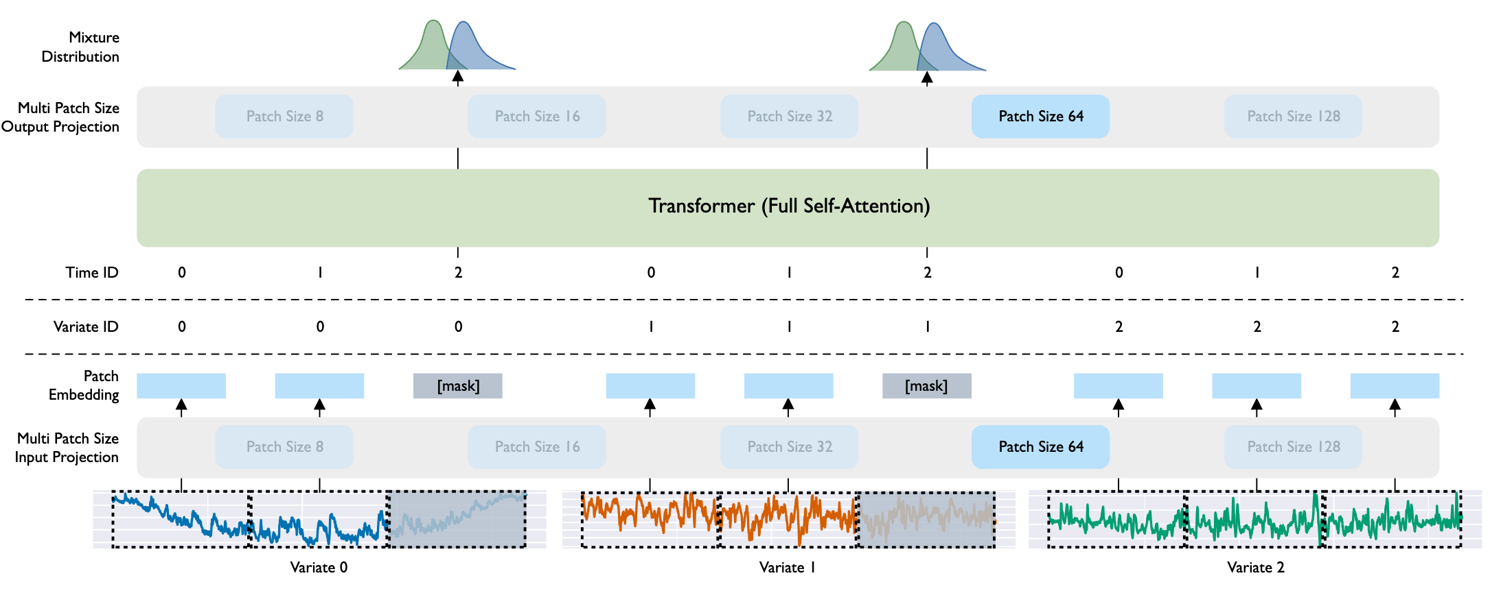
Figure 15.6: Architecture of Moirai.

Moirai is an encoder-only transformer model developed by Salesforce. It is a probabilistic model that also relies on patching the input series. It supports both historical and future exogenous variables. A distinct feature of Moirai is that it uses a mixture distribution, using four different distributions, to output more flexible prediction intervals. Its release also comes with LOTSA, an open archive of time series data with 27B data points.

For more information:

Chronos

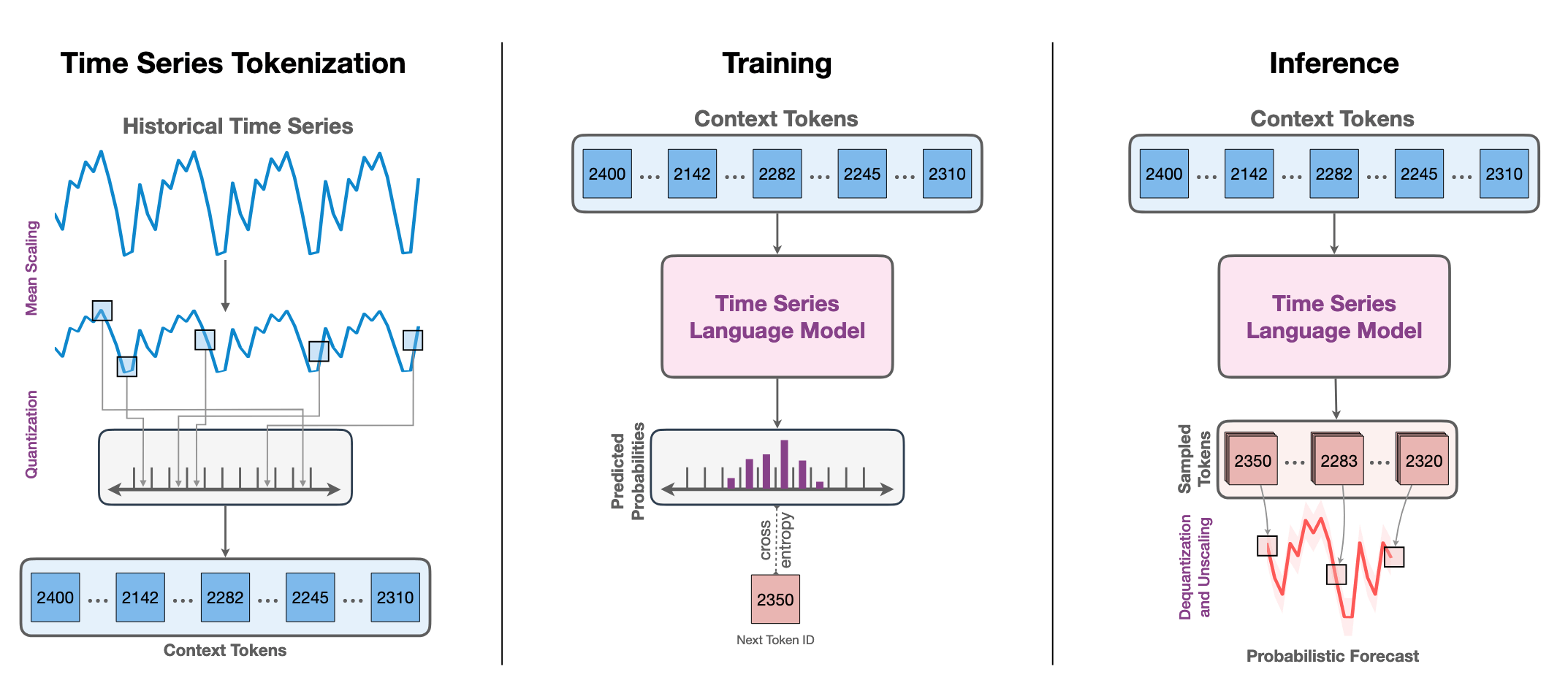
Figure 15.7: Architecture of Chronos.

Chronos is technically a framework to repurpose a large language model (LLM) for time series forecasting developed by Amazon. The researchers have pre-trained models based on the T5 family that can be used for zero-shot forecasting. The framework involves tokenising time series data points, by scaling the data and performing quantisation to create a fixed “vocabulary” of time, such that it can be used directly with LLMs. Since LLMs are by default probabilistic models, this results in a probabilistic forecasting model as well.

For more information:

15.4 Example: electricity price forecasting

In this example, we predict day-ahead electricity prices with foundation models. We use TimeGPT, which does not require local model weights, and Moirai, one of the few foundation models that supports exogenous features.

The dataset contains data from five electricity markets, each with unique price dynamics, including varying frequencies and occurrences of negative prices, zeros, and price spikes. Since electricity prices depend on exogenous factors, each dataset includes two additional time series: day-ahead forecasts of two significant exogenous factors specific to each market.

This dataset includes hourly prices (y), day-ahead forecasts of load (Exogenous1), and wind generation (Exogenous2). It also includes one-hot encoding (Section 7.4) to indicate the day of the week. For example: Monday (day_0 = 1), Tuesday (day_1 = 1), and so on.

For simplicity, we focus on the Nord Pool electricity market (NP), which represents the Nordic countries’ exchange.

df = pd.read_csv("data/electricity_short.csv", parse_dates=["ds"])
df
unique_id ds y Exogenous1 Exogenous2 day_0 day_1 day_2 ...
0 NP 2018-10-15 2.2 34078 1791 1 0 0 ...
1 NP 2018-10-15 4.0 33469 1489 1 0 0 ...
2 NP 2018-10-15 4.9 33313 1233 1 0 0 ...
3 NP 2018-10-15 10.5 33535 1035 1 0 0 ...
... ... ... ... ... ... ... ... ...
1676 NP 2018-12-23 55.6 57002 525 0 0 0 ...
1677 NP 2018-12-23 54.0 55990 478 0 0 0 ...
1678 NP 2018-12-23 53.9 54336 410 0 0 0 ...
1679 NP 2018-12-23 52.3 51679 371 0 0 0 ...

TimeGPT is offered by Nixtla as a service and can be used through an API. Nixtla offers free access for academics, students, and researchers. To create an account and generate the API key, visit their website. For specific details on the API, visit the documentation.

nixtla_client = NixtlaClient(api_key="YOUR_API_KEY")
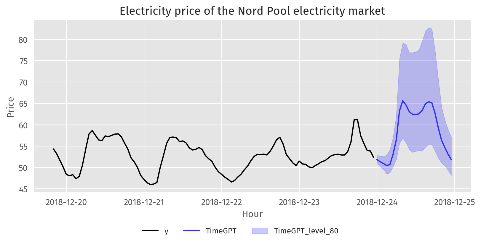
preds_df = nixtla_client.forecast(df=df, h=24, level=[80, 90])
preds_df.head()
unique_id ds TimeGPT TimeGPT
hi
80
TimeGPT
hi
90
TimeGPT
lo
80
TimeGPT
lo
90
0 NP 2018-12-24 00:00:00 51.9 52.9 53.5 50.9 50.4
1 NP 2018-12-24 01:00:00 51.4 52.6 53.1 50.3 49.8
2 NP 2018-12-24 02:00:00 51.0 52.6 53.5 49.5 49.1
3 NP 2018-12-24 03:00:00 50.5 52.9 53.9 48.5 48.0
4 NP 2018-12-24 04:00:00 50.7 54.1 54.9 48.7 48.2
plt.rcParams["figure.figsize"] = (8, 4)
plot_series(df, preds_df, level=[80],
    max_insample_length=100, xlabel="Hour", ylabel="Price",
    title="Electricity price of the Nord Pool electricity market",
    palette="black_and_blue", rm_legend=False,
    legend_loc="outside lower center")

Figure 15.8: Zero-shot forecasting with TimeGPT.

Next, we use cross-validation to evaluate the accuracy of the predictions over the last three windows.

cv_preds_df = nixtla_client.cross_validation(df=df, h=24, n_windows=3)
cv_preds_df.head()
unique_id ds cutoff y TimeGPT
0 NP 2018-12-21 00:00:00 2018-12-20 23:00:00 47.2 48.0
1 NP 2018-12-21 01:00:00 2018-12-20 23:00:00 46.4 47.4
2 NP 2018-12-21 02:00:00 2018-12-20 23:00:00 46.0 47.0
3 NP 2018-12-21 03:00:00 2018-12-20 23:00:00 46.1 46.8
4 NP 2018-12-21 04:00:00 2018-12-20 23:00:00 46.5 47.5
def transform_evaluation(evaluation):
    return (
        evaluation
        .assign(metric=lambda x: x["metric"].str.upper())
        .drop(columns=["unique_id", "cutoff"])
        .melt(id_vars='metric', var_name='Method')
        .groupby(["metric", "Method"], as_index=False)
        .agg({"value": "mean"})
        .pivot(index="Method", columns="metric", values="value")
        .reset_index().rename_axis("", axis="columns")
    )

evaluation = transform_evaluation(
    evaluate(cv_preds_df, models=["TimeGPT"], metrics=[mae])
)
evaluation
Method MAE
0 TimeGPT 1.100

Without fine-tuning, TimeGPT achieves an average MAE of 1.902.

Fine-tuning

One important characteristic of foundation models is their ability to be fine-tuned to specific datasets. This can be done with TimeGPT using the finetune_steps argument. We can also specify the finetune_loss argument to optimise a specific performance metric. In the example, we optimise for the mean absolute error (MAE).

cv_finetune_preds_df = nixtla_client.cross_validation(
    df=df, h=24, n_windows=3,
    finetune_steps=15, finetune_loss="mae")
evaluation = transform_evaluation(
    evaluate(cv_finetune_preds_df, models=["TimeGPT"], metrics=[mae])
    .rename(columns={"TimeGPT": "TimeGPT-finetuned"})
)
evaluation
Method MAE
0 TimeGPT
finetuned
1.107

With finetuning, the MAE improved to 1.895. Finetuning is usually a good approach to improve the performance of a foundation model on a particular dataset.

Incorporating exogenous variables

Until now, the model has used the historical values of the exogenous variables. However, it is beneficial for the model to provide the values of exogenous features over the forecast horizon (see Section 7.4 on predictors for regression models).

future_ex_vars_df = pd.read_csv(
  "data/electricity_future_vars.csv", parse_dates=["ds"]
)
future_ex_vars_df
unique_id ds Exogenous1 Exogenous2 day_0 day_1 day_2 ...
0 NP 2018-12-24 49119 461 1 0 0 ...
1 NP 2018-12-24 48115 484 1 0 0 ...
2 NP 2018-12-24 47727 497 1 0 0 ...
3 NP 2018-12-24 47673 509 1 0 0 ...
... ... ... ... ... ... ... ...
20 NP 2018-12-24 51787 2785 1 0 0 ...
21 NP 2018-12-24 51488 2919 1 0 0 ...
22 NP 2018-12-24 50928 3119 1 0 0 ...
23 NP 2018-12-24 49889 3306 1 0 0 ...
exog_preds_df = nixtla_client.forecast(
    df=df, X_df=future_ex_vars_df, h=24, level=[80])
columns = exog_preds_df.columns.str.replace("TimeGPT", "TimeGPT-exog")
exog_preds_df = exog_preds_df.set_axis(columns, axis="columns")
exog_preds_df.head()
unique_id ds TimeGPT
exog
TimeGPT
exog
hi
80
TimeGPT
exog
lo
80
0 NP 2018-12-24 00:00:00 51.4 53.0 50.2
1 NP 2018-12-24 01:00:00 50.3 52.2 48.9
2 NP 2018-12-24 02:00:00 49.7 52.3 47.8
3 NP 2018-12-24 03:00:00 49.4 52.5 47.1
4 NP 2018-12-24 04:00:00 49.8 54.0 47.1
fcst_df = preds_df.merge(exog_preds_df)
plot_series(df, fcst_df,
    max_insample_length=100, xlabel="Hour", ylabel="Price",
    title="Electricity price of the Nord Pool electricity market",
    palette="black_and_2color", rm_legend=False,
    legend_loc="outside lower center")

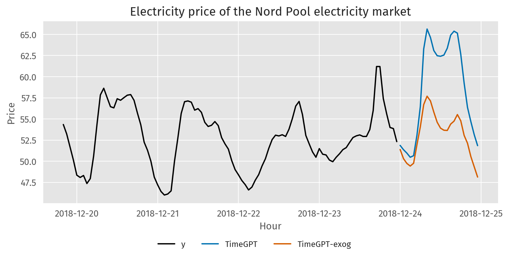
Figure 15.9: Forecasting with exogenous features with TimeGPT.

In Figure 15.9, we can see that by using exogenous features, the model can model variations in the data that were not previously captured.

As mentioned before, Moirai is also a foundation model that supports the use of exogenous variables. First, we start by converting the dataset to a GluonTS dataset.

full_df = pd.concat([df, future_ex_vars_df], axis=0)
full_df = full_df.set_index("ds")
ds = PandasDataset.from_long_dataframe(
    full_df,
    target="y",
    item_id="unique_id",
    feat_dynamic_real=full_df.columns.drop(["unique_id", "y"]).tolist(),
)

To keep things consistent, we keep the forecast horizon to 24 time steps into the future.

train, test_template = split(ds, offset=-24)
test_data = test_template.generate_instances(
    prediction_length=24, windows=1, distance=24,
)

Then, we initialise the Moirai model. We can choose between small, base and large. Here, let’s use the large model. The model weights are downloaded from Hugging Face Hub. If you encounter rate-limit or authentication errors, set a Hugging Face token first (a free account is sufficient).

model = MoiraiForecast(
    module=MoiraiModule.from_pretrained(f"Salesforce/moirai-1.0-R-large"),
    prediction_length=24,
    context_length=240,
    patch_size="auto",
    num_samples=50,
    target_dim=1,
    feat_dynamic_real_dim=ds.num_feat_dynamic_real,
    past_feat_dynamic_real_dim=ds.num_past_feat_dynamic_real,
)

Once the model is initialised, we can use it for zero-shot forecasting with the available exogenous features.

predictor = model.create_predictor(batch_size=32)
forecasts = list(predictor.predict(test_data.input))
fc = forecasts[0]
moirai_preds_df = (
    pd.DataFrame(np.quantile(fc.samples, [0.5, 0.1, 0.9], axis=0).T)
    .set_axis(["Moirai", "Moirai-lo-80", "Moirai-hi-80"], axis="columns")
    .assign(ds=fc.index.to_timestamp())
)

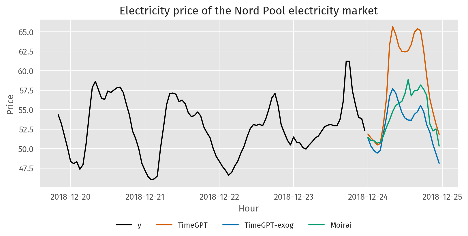
Since Moirai is a probabilistic model, it returns a distribution of future values. Thus, let’s take the median as the point forecast.

fcst_df = preds_df.merge(exog_preds_df).merge(moirai_preds_df)
plot_series(df, fcst_df, max_insample_length=100,
    xlabel="Hour", ylabel="Price",
    title="Electricity price of the Nord Pool electricity market",
    palette="black_and_3color", rm_legend=False,
    legend_loc="outside lower center")

Figure 15.10: Forecasting with exogenous features with TimeGPT and Moirai.

15.5 Further reading

  • A benchmark by Nixtla of the foundation models discussed in this chapter, available here.
  • A review of the current state and future prospects of LLMs and Foundation Models in forecasting can be found in Bergmeir (2024).
  • Another recent benchmark from Salesforce is Aksu et al. (2024).
  • A comprehensive survey of foundation models is Liang et al. (2024).

If you want to learn more about a benchmark of the foundation models discussed in this chapter, consult this experiment here.

15.6 Used modules and classes

NixtlaClient

  • NixtlaClient class - Core client for accessing TimeGPT API

NeuralForecast

  • NeuralForecast class - Framework for neural forecasting models
  • NHITS model - Neural hierarchical interpolation for time series model

UtilsForecast

  • plot_series() utility - For creating time series visualisations
  • evaluate() utility - For model evaluation